

How Much Poorer Will Climate Change Make Us?
How Much Poorer Will Climate Change Make Us?


This is a difficult question to answer, but an important one. The answer can (or should) guide our decisions on which climate change mitigation policies are worth doing.
Economists Adrien Bilal and Diego Känzig recently released a study in which they find that, when the average temperature on earth goes up by 1°C, global gross domestic product (GDP) declines by 12%. Based on this number, they estimate that burning a gallon of gasoline costs the world $9.40 in climate damages ($1056 per ton of carbon dioxide). That is a really big number.
In this article, I describe how researchers come up with numbers like this. In many ways, it's not complicated, but it can seem mystical to the uninitiated. In the process, you'll see some skepticism about this particular estimate of the effect of temperature on GDP. If at any point you get lost in the details, just skip to the conclusion for the TLDR.
This blog is called Ag Data News because most of what I write fits those three labels. This week's article is a little different because it is not about agriculture, although the first major empirical studies of the effect of climate change on the economy were about agriculture (e.g., here and here).
GDP vs Temperature
Following Bilal and Känzig, let's look at data on global average temperature and compare it to global GDP. This is what economists call a reduced form analysis. We won't model how the temperature affects GDP; we will just look at how the two variables relate to each other. I won't get to Bilal and Känzig's model until near the end. Click here to see my R code.
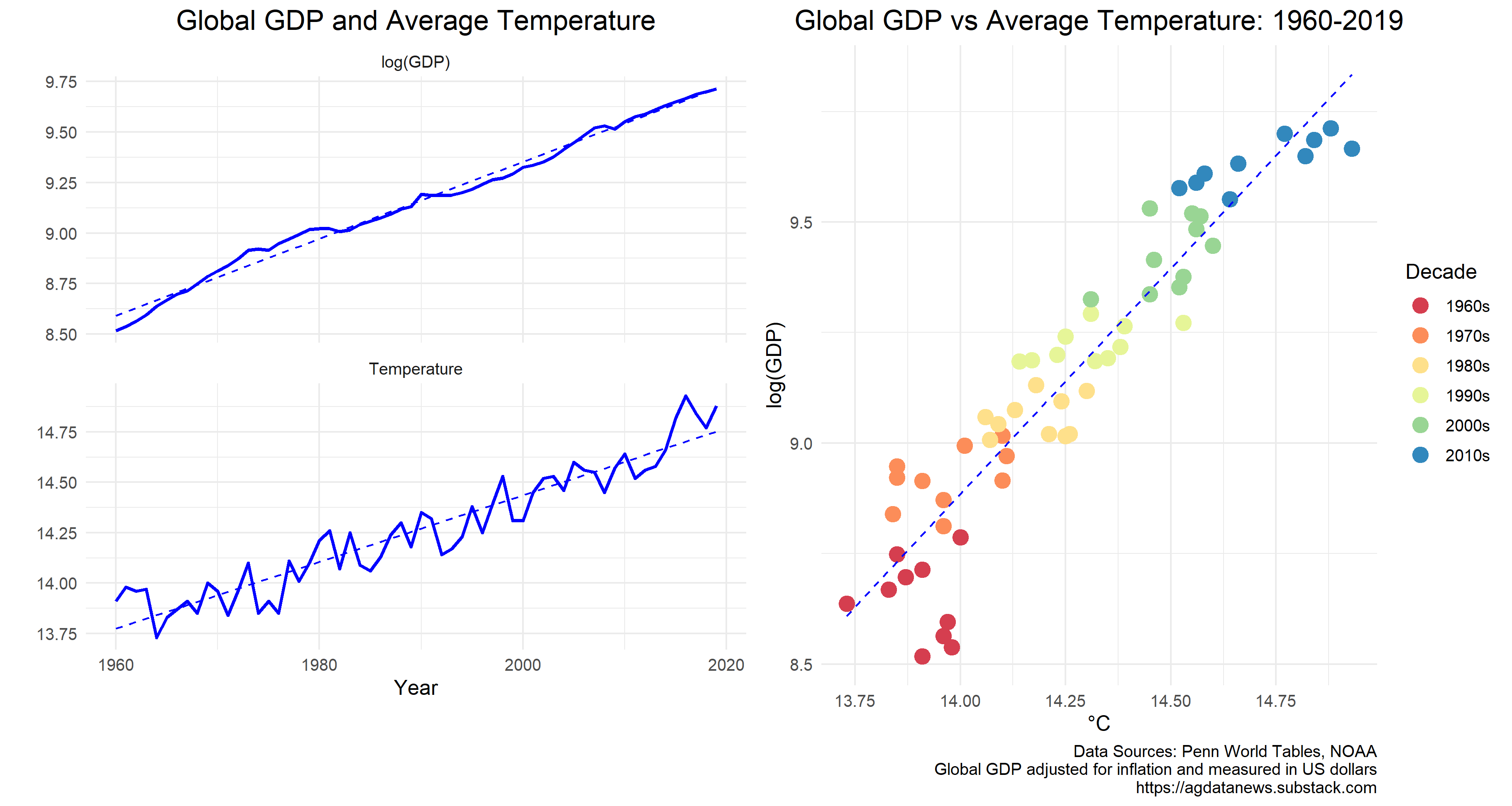
The graph above shows GDP and temperature since 1960. GDP is measured in natural logarithms so that 0.1 units corresponds to about 10%. Temperature is measured in degrees Celsius.
Both variables have gone up over time. The line of best fit between the two variables is:
which implies that GDP has increased about 10% for every 0.1 degree increase in temperature. Does this mean that the increasing temperature is causing GDP to increase? Common sense says no. This simple equation doesn't account for the main drivers of GDP growth, such as new technology and population growth.
So, let's accept that the global economy was going to grow whatever happened to the temperature. On average from 1960 through 2019, GDP grew at 1.9% per year and temperature grew by 0.017° per year. What if we remove the trend from the data? If the temperature was above its trend line one year, was GDP below its trend line that year?
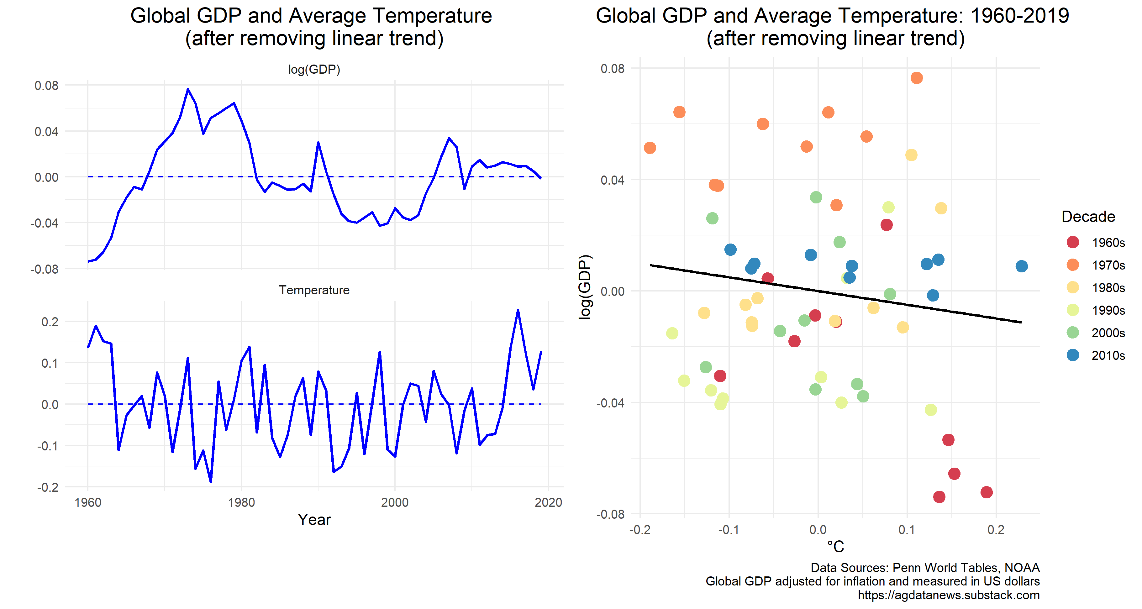
The graph above shows the the two series after subtracting out their trend lines. GDP was below trend until the mid 1960s and above trend through the 1970s. Temperature was above trend until the mid 1960s and below trend through the 1970s.
The line of best fit for the detrended data is:
which implies that GDP tended to be 5% below trend when temperature was 1°C above trend. The 95% confidence interval for this estimate is [-18.2%, 8.3%], which is a very wide range (Technical note: I adjusted the standard errors for autocorrelation using the Newey-West estimator with pre-whitening and 3 lags.)
Does this mean that an extra degree causes GDP to drop by 5%? Again, I would say no. First, the confidence interval includes zero, so statistically we can't rule out a zero relationship. Second, GDP typically departs from its trend for a decade or more, but it stretches credulity to claim that climate is the cause. Can we really attribute the booming 1970s to below-trend temperatures?
OK, let's get serious
The problem here is that GDP is related to past values of itself. Good years tend to follow good years and vice versa. To capture the incremental effect of temperature on GDP, we need to separate the inertia of GDP from events that divert it to a different path.
In 1980, Christopher Sims proposed a solution to this problem in a famous paper called "Macroeconomics and Reality". He proposed the use of vector autoregression models to measure how a set of economic variables affect each other over time. Sims won the Nobel prize for economics in 2011.
In our context, the Sims approach would entail three steps:
Predict GDP and temperature over the next several years based on recent values of GDP as well as a linear trend and current and past temperatures.
Predict GDP again, except assume that this years temperature was one degree higher than the model had predicted.
Take the difference between the two GDP forecasts.
This difference is known as an impulse response; it is the incremental effect of an extra degree this year on expected GDP in future years.
The key insight is that getting hit by higher-than-expected temperature is like an experiment. The impulse response shows how GDP tends to respond to such experiments.
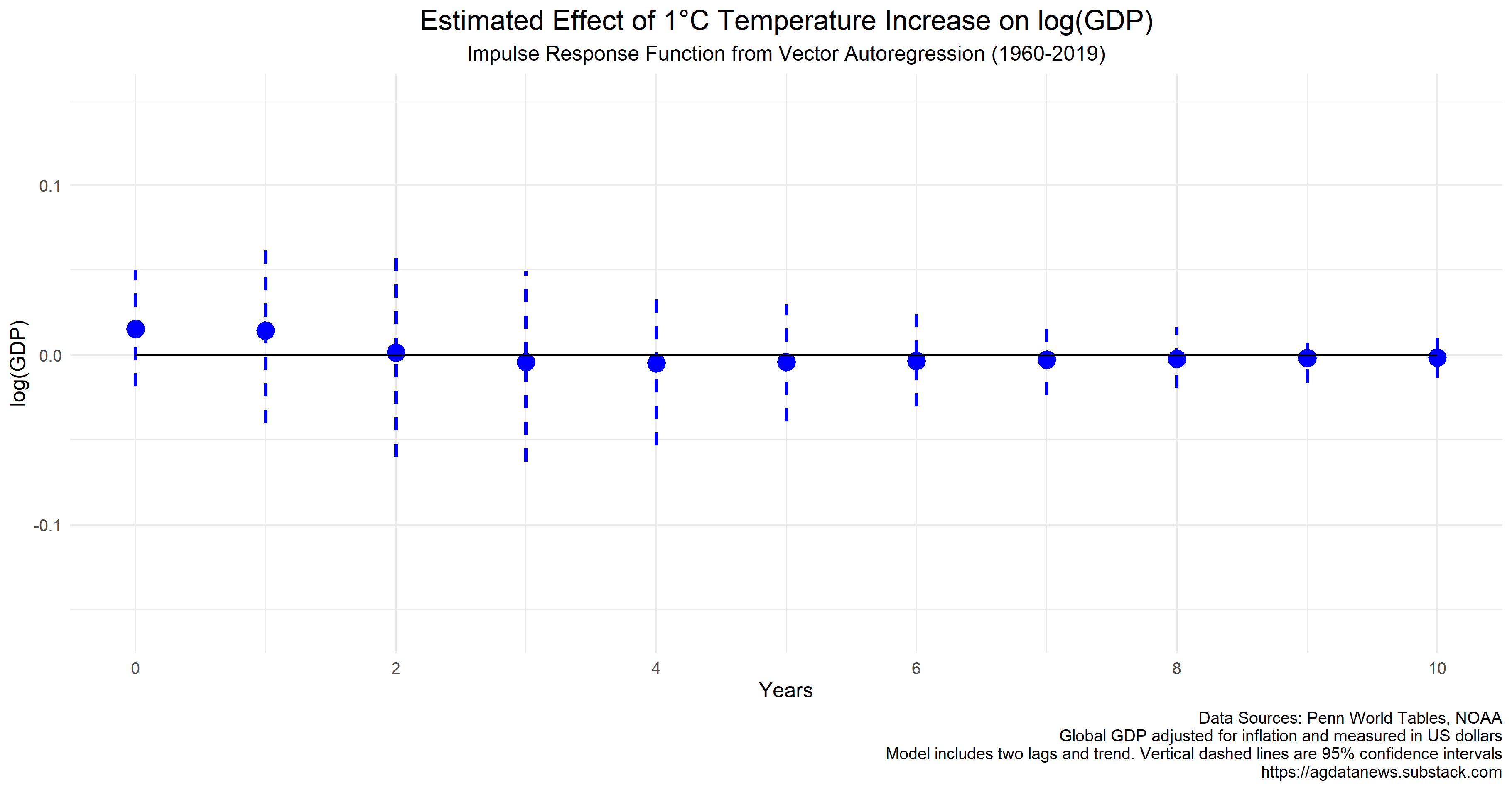
Using this approach produces a small positive impulse response of GDP to a higher temperature in the same year, and very small negative response in subsequent years as shown in the above chart. In subsequent years, the effect of this temperature shock subsides. Importantly, the response is not statistically significant at any horizon.
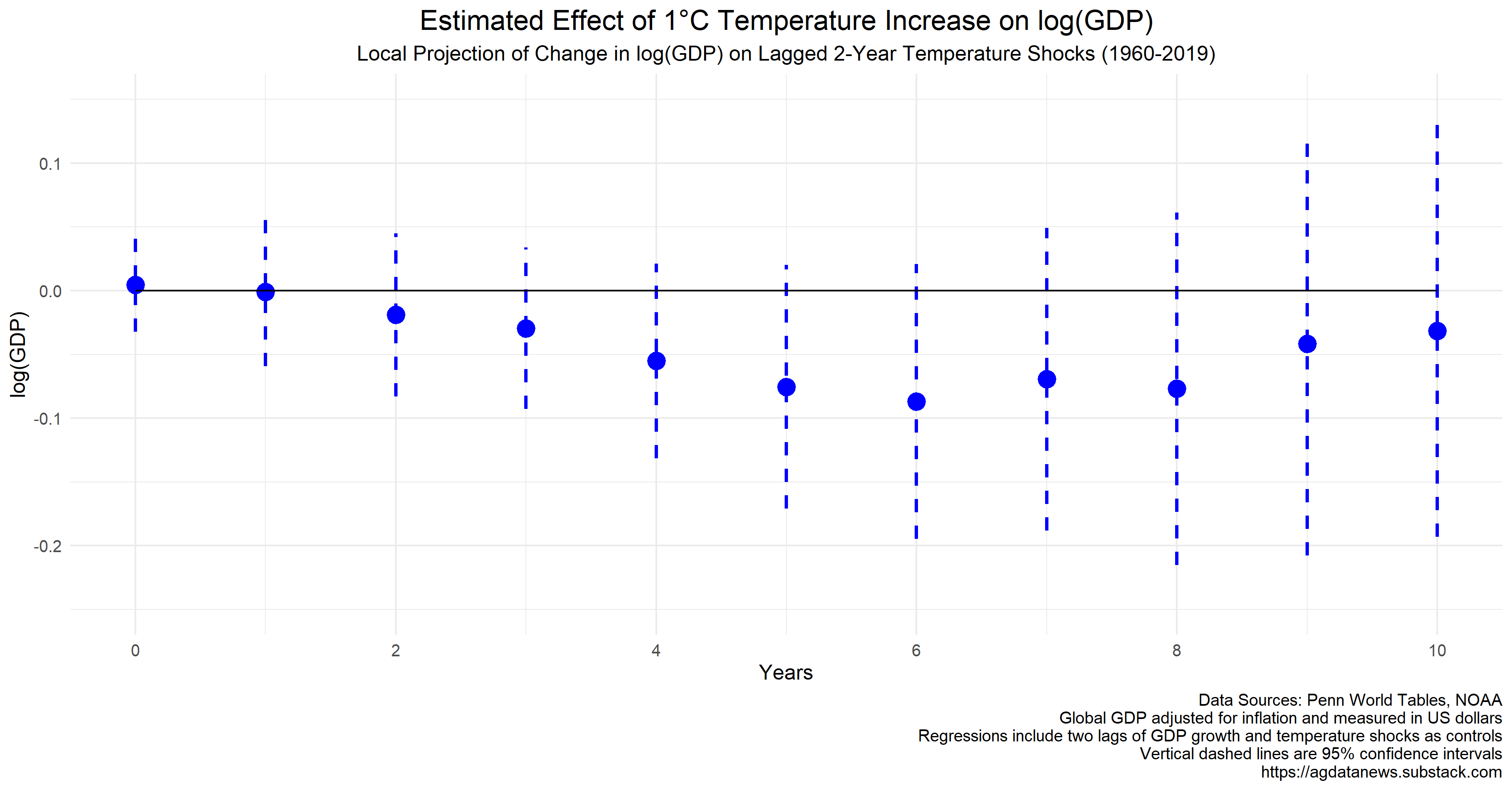
In 2005, my UC Davis colleague Òscar Jordà came up with a simpler and more flexible method for estimating impulse responses. Instead of one big model, use a separate model for each forecast horizon. To estimate how a surprising one-degree increase in temperature affects GDP, say, five years from now, just fit a model relating GDP to temperature five years ago. Use the values of GDP and temperature from six and seven years ago as controls to handle the inertia problem. He called this method local projections.

Local projections produce similar results to Sims' vector autoregression at short horizons and slightly different results at longer horizons. This result highlights the differences in the methods. The vector autoregression extrapolates the nearby relationships to infer the distant relationships, whereas local projections estimates each relationship directly.
Five years after the temperature shock, the local projections model predicts GDP would be 3.3% lower than it would have been, but this effect is not statistically different from zero.
Jordà's local projections approach built a bridge from Sims vector autoregression to the new econometrics of the so-called credibility revolution, which emphasizes using better data and techniques to distinguish correlation from causation. David Card, Guido Imbens, and Joshua Angrist won the Nobel Prize in 2021 for their pioneering work in this area. In many cases, choosing data wisely allows researchers to estimate causal effects using the multiple regression models that undergraduates learn in their first econometrics class. In fact, I worked through this temperature and GDP problem with my ARE 106 class this past quarter.
So far in my analysis, I have used a straight-line trend, but it is not be the best model for these data. The annual rate of GDP growth is not a constant 1.9% (we cannot reject the null hypothesis of a unit root against trend stationarity). Temperature looks pretty flat until the mid 1970s, before starting its upward trend.
This brings us to Bilal and Känzig. They use Jordà's local projections method but with different variables. For GDP, they focus on year-to-year changes. For temperature, they first predict it based on its own past and then use the difference between actual and predicted temperature in the models.
The temperature step is important, so I'm going to show you the math. They predict temperature in year t using temperature in years t-2 and t-3 and get the following model:
The prediction errors are the surprise (or shock) component of this year's temperature relative to what we knew two years ago, i.e., actual minus predicted:
Here’s what the data look like:

Each temperature shock is like a two-year experiment. To estimate how temperature shocks affect GDP, fit a regression model to predict GDP in future years as a function of this year's shock and historical controls, e.g., for predicting five years ahead, the model is:
(Note: The variable ΔGDP(t-1) is the change in log GDP from year t-2 to year t-1. Bilal and Känzig use data from 1950-2022 to estimate the shocks and 1960-2019 to estimate the effects of the shocks on GDP. The numbers in these equations are from linear regression models estimated by ordinary least squares.)
The above impulse responses are similar to those from the Jordà method, although they have shifted down. They show no contemporaneous effect, and a negative but statistically insignificant effect after a few years. (Defining the shock based on a prediction made one year ago instead of two produces almost identical results, which is to be expected given that both models include lagged shocks as controls.)
Bilal and Känzig also include in their model indicator variables for global recessions. Their idea is that an El Niño event could increase temperature and precipitate a recession, and they don't want to attribute the economic downturn to a climate shock. They define a recession indicator variable that equals one in 1973-1975, 1979-1983, 1990-1992, and 2007-2009, and zero otherwise. They include the recession indicator and its first two lags as controls.

With this change, we get more negative effects of temperature on GDP. We continue to see a negligible contemporaneous response, but the response in later years becomes larger and statistically significant, reaching 9.5% in year 5 and peaking at 10.8% in year 6. This figure matches Figure 3 in Bilal and Känzig's paper. The argument for adding the recession indicator variables was that without them the estimated effect may be too large, so we should have seen smaller and not larger estimates after adding the recession variables.
Conclusion
Using data from the last 60 years, modern econometric methods reveal that global GDP drops after a surprise increase in the global average temperature. This drop occurs several years after the temperature shock. However, confidence intervals for the magnitude of this drop are wide. In many versions of the model, the confidence interval includes zero, which means the model cannot rule out a zero relationship.
This is not a criticism of Bilal and Känzig’s analysis. You can only do so much with 60 years of data. Bilal and Känzig use panel data methods to improve precision (i.e., estimate each country’s GDP response to global temperature shocks), but their confidence intervals remain wide.
One implication of wide confidence intervals is that the estimated effect can be sensitive to seemingly small changes in the model. For example, tinkering with the year I begin the sample and the way I control for recessions moves the estimates around (see below). The shape of the curves is pretty stable, but the estimated effect at a 5 year horizon ranges from 2.2% to 13.1%.

Does it make sense that GDP has little if any response to a temperature shock in the year it happens, but instead declines several years later? This is Bilal and Känzig’s key finding, and validating it will require detailed analysis of how it occurs. They present some evidence that shocks to global average temperature portend “future extreme weather events such as storms that materialize as a sequence of capital depreciation shocks.”
A recent paper by Martin Bodenstein and Mikaël Scaramucci estimates directly the effect of natural disasters on GDP and finds that severe weather events predict significant GDP declines several years after the event, especially in middle income countries and especially for major droughts and forest fires. Bilal and Känzig also find the largest effects in middle income countries.
In sum, it seems plausible that these papers are picking up sustained economic effects of extreme weather events that are associated with climate change. The possible magnitude of these effects ranges from small to massive.
Addendum
There are other points to debate regarding what this study tells us about the GDP effects of climate change. Among them are:
The temperature shocks in this study are mostly between -0.2°C and 0.2°C. Climate change will bring larger shocks over a longer period of time.
People will adapt to the changing climate, so after a while the effects of hot temperatures will decline.
It's not all about the money. Reduced quality of life and loss of biodiversity are examples of climate damages that may not show up in the GDP numbers.
I did the analysis in this article using this R code. Thanks to Diego Känzig for thoroughly answering my questions about their analysis.